
BrewMonitor: A Look at Fermentation Data Curves – Conductivity Examples

BrewMonitor® offers your brewing team access to insight that has never been available before: high-resolution data from inside your fermentation tank, allowing you to track the progress of your fermentation, analyze results, benchmark future batches, and much more. The resulting graphs for each completed fermentation – dissolved oxygen, pH, gravity, pressure, temperature and conductivity – provide extremely clear views into the events that transpired and techniques that were employed.
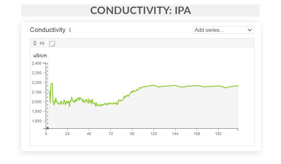
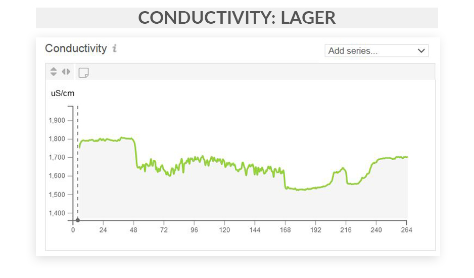
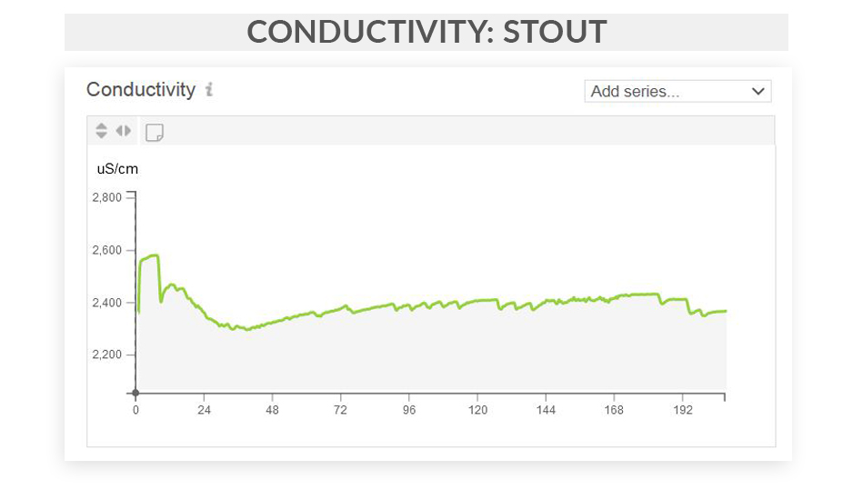
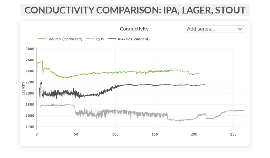
This series of articles shows examples of data curves from specific parameters, as they were recorded from the fermentation of various styles in different scenarios. These graphs are from actual fermentations, and offered as a look into how these conditions express themselves as measured data trends. In this installment, we step through some examples of typical conductivity curves.
See our earlier post on typical gravity curves »
See our earlier post on typical pH curves »
Free eBook: Leveraging Data-Driven Fermentation Performance Management

Can fermentation management be improved, as a process? This eBook explores, in detail, how fermentation performance data analysis helps elevate product and business outcomes in a modern brewery, whether brewpub, microbrewery or regional craft brewer.
You will learn:
- Day-by-day performance considerations – learned through the extensive examination of real-time fermentation tank data.
- Key recommendations from the Precision Fermentation science team at each major step of fermentation – “Day zero” (i.e. before you pitch your yeast), the first 24 hours, and day two through the end of fermentation.
- Best practices – Activity to watch out for, broken down by each key measurement – Dissolved oxygen, gravity, pH, pressure, internal/external temperature, and conductivity.
- Key findings that can help you solve problems and improve your results.